This article explains spectrogram of the speech signal (analysis and processing) with MATLAB to get its frequency-domain representation.
In real life, we come across many signals that are variations of the form ƒ(t), where ‘t’ is independent variable ‘time’ in most cases. Temperature, pressure, pulse rate, etc can be plotted along the time axis to see variations across time.
In signal processing, signals can be classified broadly into deterministic signals and stochastic signals. Deterministic signals can be expressed in the form of a mathematical equation and there is no randomness associated with them. The value of the signal at any point of time can be obtained by evaluating the mathematical equation. An example is a pure sine wave:
ƒ(t)=A sin 2πƒt
where ‘A’ is signal amplitude, ‘ƒ’ is signal frequency and ‘t’ is time.
Many of the information-bearing signals may not be predictable in advance. There is a certain amount of randomness in the signal with respect to time. Such signals cannot be expressed in the form of simple mathematical equations. For example, in the noise signal inside a running automobile, we may hear many sounds, including the engine sound, sound of horns from other vehicles and passengers talking, in a combined form with no predictability. Such signals are examples of stochastic signals.
In the speech signal produced when you utter steady sounds like ‘a,’ ‘i’ or ‘u,’ the waveform is a near-periodic repetition of some well-defined patterns. When you produce sounds like ‘s’ and ‘sh,’ the waveform is noise-like. The periodicity in the speech signal is due to the vibration of vocal folds at a particular frequency, known as pitch or fundamental frequency of the speaker. Steady sounds (a, i or u) are examples of vowels and noise-like sounds (s and sh) are examples of consonants. Human speech signal is a chain of vowels and consonants grouped in different forms.
Most of the signals in real life are available continuously and may assume any amplitude value. These signals are called analogue signals and they are not in a form suitable for storing or processing using a digital computer. In digital signal processing, we process the signal as an array of numbers. We do sampling along the time axis to discretise the independent variable ‘t.’ In other words, we look at the signal at a number of time instances separated by a fixed interval ‘T’ (called sampling period==1/ƒs, where ‘ƒs’ is called sampling frequency). Signal values observed at these time instances are further discretised in the amplitude domain to make these suitable for storage in the form of binary digits. This process is called quantisation. After sampling and quantisation (called digitisation) of an analogue signal, the signal assumes the form:
ƒ(n)=qn
where ‘qn’ is an approximation to the signal amplitude at time instant t=nT. The signals so produced are called digital signals. These can be stored in memory and used for processing by mathematical operations with the help of digital computers.
A pure sine-wave after digitisation can be represented as an array in the form:
ƒ(n)=A sin 2πƒnT=A sin 2πƒn/ƒs
where ‘A’ is the signal amplitude, ‘ƒ’ is the signal frequency, ‘ƒs’ is the sampling frequency and ‘n’ is an integer called time index. Sample value (n) is an approximation of the signal amplitude at time instant t=nT.
Understanding the speech signal
Record vowel sound ‘aa’ using the computer’s microphone and save it as a wav file. Select sampling frequency as 10kHz. You may use audio processing software like Praat, Audacity, Goldwave or Wavesurfer to record the signal in wav format at the required sampling frequency.
The waveform of the signal, which is a plot of the amplitude of the speech signal for each sample instant, looks like Fig. 1. The horizontal axis is time units in samples and the vertical axis is amplitude of the corresponding samples. If you record sound ‘as’ in which consonant sound ‘s’ follows the vowel sound ‘a,’ and plot the signal, the waveform may look like Fig. 2.
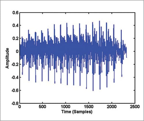
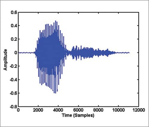
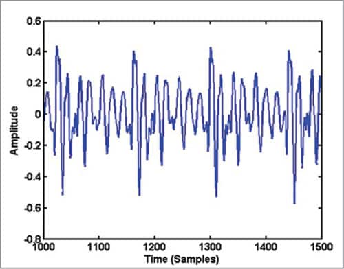
On close examination of Fig. 1, you can see some repeating pattern in it. A zoomed version of Fig. 1 showing samples in the range 1000 to 1500 is given in Fig. 3. If you plot samples from 6000 to 6500 in Fig. 2, you get Fig. 4. Obviously, the waveform in Fig. 4 has no periodicity and it appears noise-like. In the waveform of vowel-consonant sound ‘as,’ you can see that the speech signal properties transform gradually from a nearly periodic signal (samples 2000 to 5000) to a noise-like signal (samples 5000 to 10000).

This content was originally published here.